Graph Theory
Graph Theory
Graph is probably the data structure that has the closest resemblance to our daily life. There are many types of graphs describing the relationships in real life. For instance, our friend circle is a huge “graph”.

Figure 1. An example of a undirected graph.
In Figure 1 above, we can see that person G, B, and E are all direct friends of A, while person C, D, and F are indirect friends of A. This example is a social graph of friendship. So, what is the “graph” data structure?
Types of “graphs”
There are many types of “graphs”. In this Explore Card, we will introduce three types of graphs: undirected graphs, directed graphs, and weighted graphs.
Undirected graphs
The edges between any two vertices in an “undirected graph” do not have a direction, indicating a two-way relationship.
Figure 1 is an example of an undirected graph.
Directed graphs
The edges between any two vertices in a “directed graph” graph are directional.
Figure 2 is an example of a directed graph.
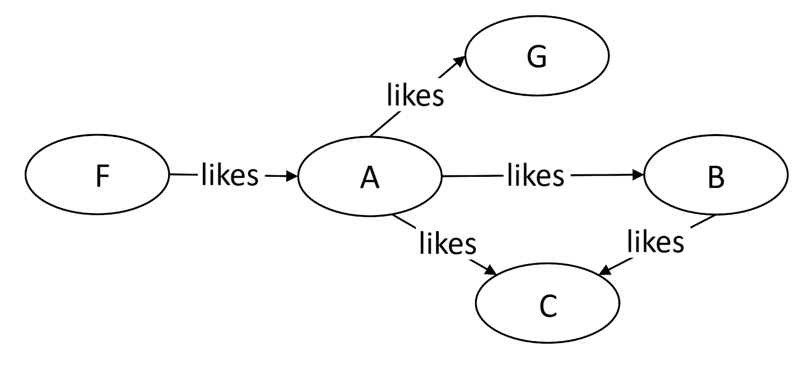
Figure 2. An example of a directed graph.
Weighted graphs
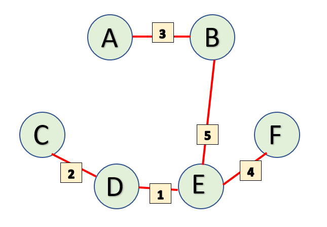
Each edge in a “weighted graph” has an associated weight. The weight can be of any metric, such as time, distance, size, etc. The most commonly seen “weighted map” in our daily life might be a city map. In Figure 3, each edge is marked with the distance, which can be regarded as the weight of that edge.
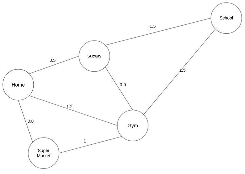
Figure 3. An example of a weighted graph.
The Definition of “graph” and Terminologies
“Graph” is a non-linear data structure consisting of vertices and edges. There are a lot of terminologies to describe a graph. If you encounter an unfamiliar term in the following Explore Card, you may look up the definition below.
- Vertex: In Figure 1, nodes such as A, B, and C are called vertices of the graph.
- Edge: The connection between two vertices are the edges of the graph. In Figure 1, the connection between person A and B is an edge of the graph.
-
Path: the sequence of vertices to go through from one vertex to another. In Figure 1, a path from A to C is [A, B, C], or [A, G, B, C], or [A, E, F, D, B, C].
Note: there can be multiple paths between two vertices.
-
Path Length: the number of edges in a path. In Figure 1, the path lengths from person A to C are 2, 3, and 5, respectively.
- Cycle: a path where the starting point and endpoint are the same vertex. In Figure 1, [A, B, D, F, E] forms a cycle. Similarly, [A, G, B] forms another cycle.
- Negative Weight Cycle: In a “weighted graph”, if the sum of the weights of all edges of a cycle is a negative value, it is a negative weight cycle. In Figure 4, the sum of weights is -3.
- Connectivity: if there exists at least one path between two vertices, these two vertices are connected. In Figure 1, A and C are connected because there is at least one path connecting them.
- Degree of a Vertex: the term “degree” applies to unweighted graphs. The degree of a vertex is the number of edges connecting the vertex. In Figure 1, the degree of vertex A is 3 because three edges are connecting it.
- In-Degree: “in-degree” is a concept in directed graphs. If the in-degree of a vertex is d, there are d directional edges incident to the vertex. In Figure 2, A’s indegree is 1, i.e., the edge from F to A.
- Out-Degree: “out-degree” is a concept in directed graphs. If the out-degree of a vertex is d, there are d edges incident from the vertex. In Figure 2, A’s outdegree is 3, i,e, the edges A to B, A to C, and A to G.
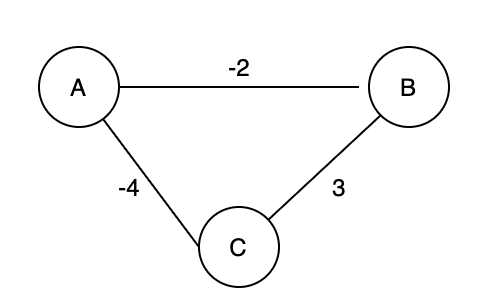
Figure 4. An example of a negative weight cycle.
Representations of Graph
Here are the two most common ways to represent a graph :
- Adjacency Matrix
- Adjacency List
Adjacency Matrix
An adjacency matrix is a way of representing a graph as a matrix of boolean (0’s and 1’s).
Let’s assume there are *n vertices in the graph So, create a 2D matrix adjMat[n][n]* having dimension n x n.
- If there is an edge from vertex *i to j, mark adjMat[i][j] as 1*.
- If there is no edge from vertex *i to j, mark adjMat[i][j] as 0*.
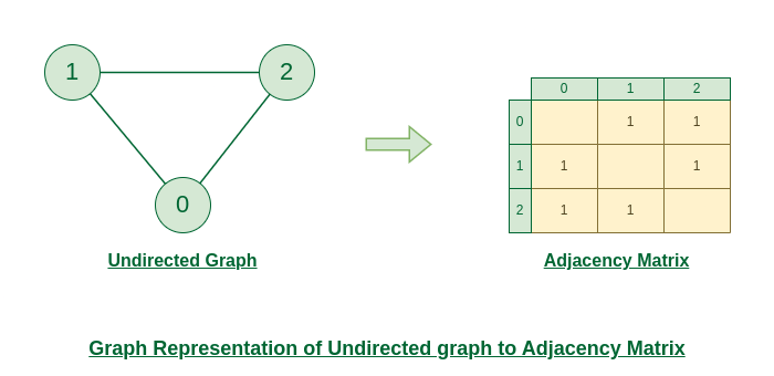
Representation of Undirected Graph to Adjacency Matrix:
The below figure shows an undirected graph. Initially, the entire Matrix is initialized to *0. If there is an edge from source to destination, we insert 1 to both cases (adjMat[destination] and adjMat[destination])* because we can go either way.
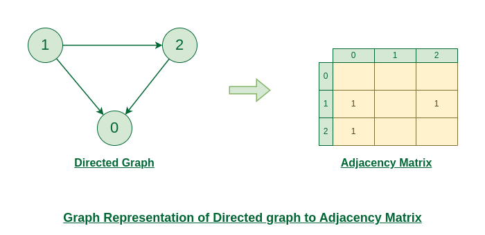
Representation of Directed Graph to Adjacency Matrix:
The below figure shows a directed graph. Initially, the entire Matrix is initialized to *0. If there is an edge from source to destination, we insert 1 for that particular adjMat[destination]*.
Adjacency List
An array of Lists is used to store edges between two vertices. The size of array is equal to the number of *vertices (i.e, n). Each index in this array represents a specific vertex in the graph. The entry at the index i of the array contains a linked list containing the vertices that are adjacent to vertex i*.
Let’s assume there are *n vertices in the graph So, create an array of list of size n as adjList[n].*
- adjList[0] will have all the nodes which are connected (neighbour) to vertex *0*.
- adjList[1] will have all the nodes which are connected (neighbour) to vertex *1* and so on.
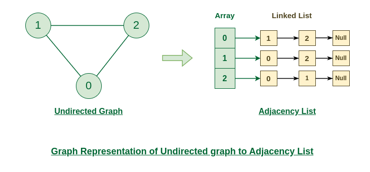
Representation of Undirected Graph to Adjacency list:
The below undirected graph has 3 vertices. So, an array of list will be created of size 3, where each indices represent the vertices. Now, vertex 0 has two neighbours (i.e, 1 and 2). So, insert vertex 1 and 2 at indices 0 of array. Similarly, For vertex 1, it has two neighbour (i.e, 2 and 1) So, insert vertices 2 and 1 at indices 1 of array. Similarly, for vertex 2, insert its neighbours in array of list.
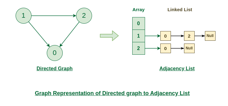
Representation of Directed Graph to Adjacency list:
The below directed graph has 3 vertices. So, an array of list will be created of size 3, where each indices represent the vertices. Now, vertex 0 has no neighbours. For vertex 1, it has two neighbour (i.e, 0 and 2) So, insert vertices 0 and 2 at indices 1 of array. Similarly, for vertex 2, insert its neighbours in array of list.
Common algorithms
BFS:
Breadth-first search (BFS) is an algorithm for searching a tree data structure for a node that satisfies a given property. It starts at the tree root and explores all nodes at the present depth prior to moving on to the nodes at the next depth level. Extra memory, usually a queue, is needed to keep track of the child nodes that were encountered but not yet explored.
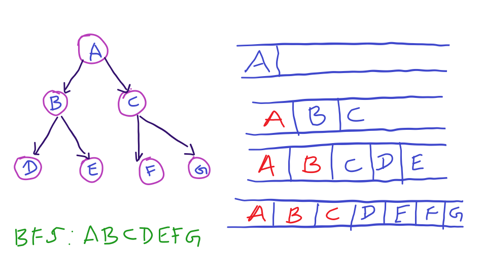
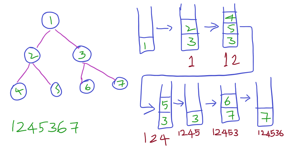
BFS is actually traversing the nodes level by level. That is, traversing the node first, then its children and then its children’s children. If you consider the following tree,
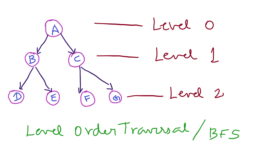
The root node is A. Its left and right children are B and C. Further its children are D,E,F and G. So the BFS of the above tree is
ABCDEFG
Here Level Order traversal of a tree is going to be same as BFS since it traverse starting from level 0 till its last level. But not every BFS is level order traversal. For example,
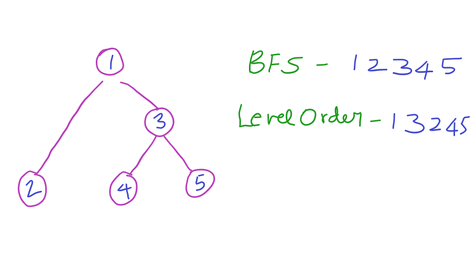
Here the BFS traverse its left and right children first and then its children.
So the BFS traversal of the above tree is 12345. Whereas Level Order traverse level by level. So the level order traversal of the same tree is 13245.
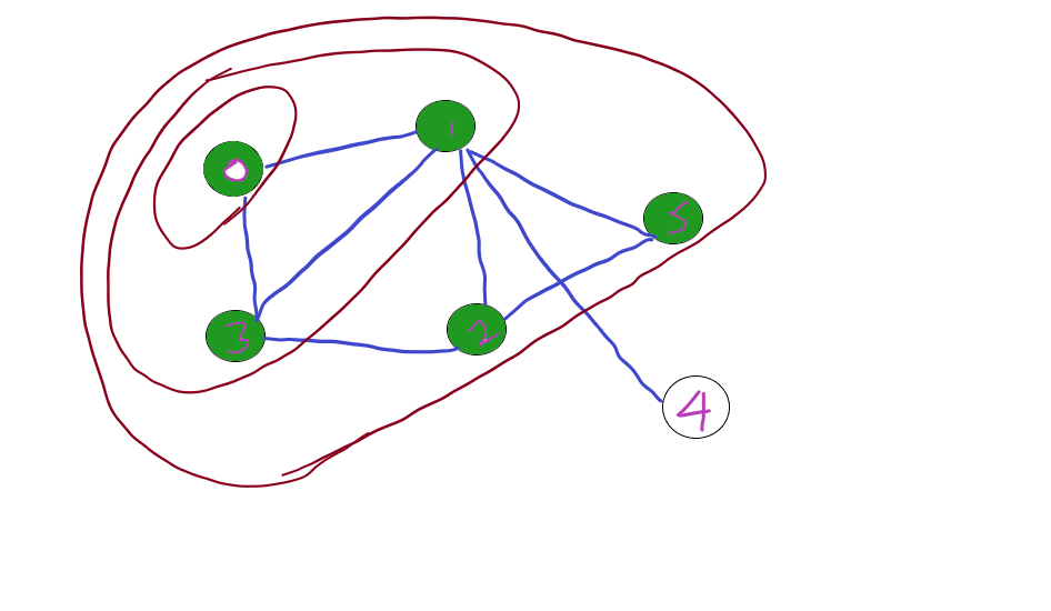
Traversing the graph in BFS way is again going to be same. That visiting the nodes wider as the graph goes.
Consider the following graph,
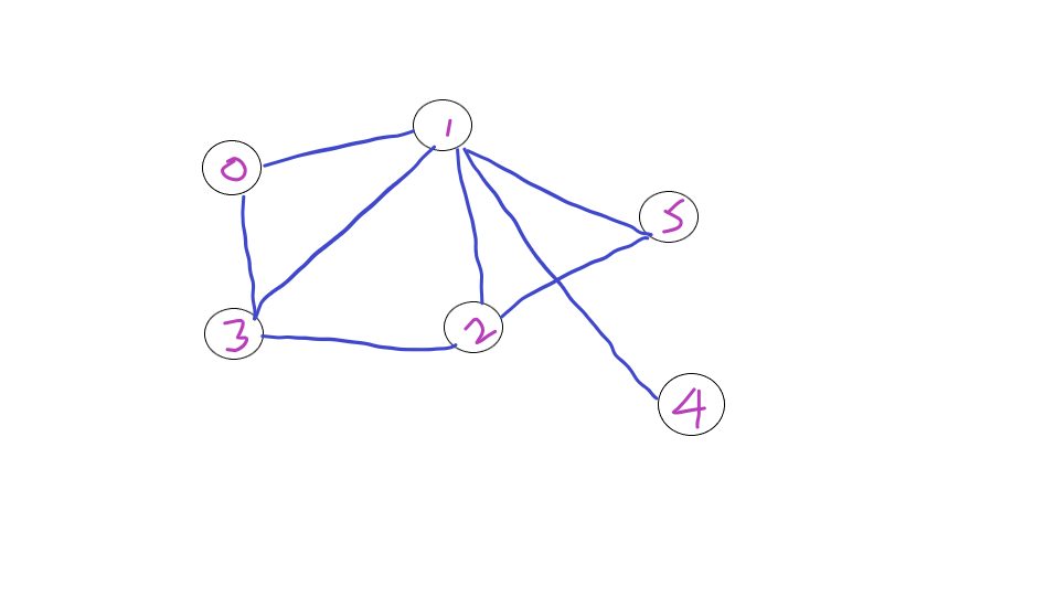
Let’s traverse starting from Node 0, we first visit 0 and traversing its neighbouring nodes 1 and 2.
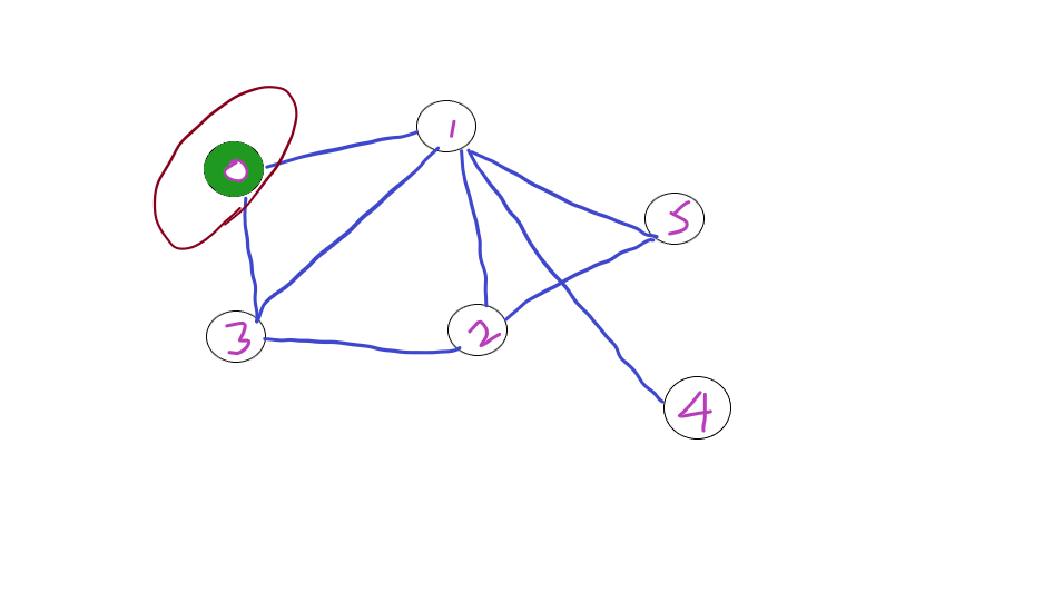
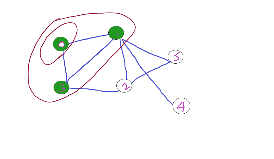
Further traversing the next wider level 2 and 5. And Finally 4.
Implementation:
BFS: FIFO (First In First Out)
In Breadth-First-Search, queue is going to be our hero. Here are the steps to implement BFS programmatically.
- Put the visited node in queue.
- Explore its children, add them to queue, and remove the visited node.
- Visit all the nodes until queue becomes empty.
In the above tree,
- we first put the root node A in queue. A’s children are B and C. Add them to queue and remove A.
- Further pull B, add its children D and E to queue and remove B.
- Pull C, add its children F and G to queue and remove C.
- D,E,F and G have no children, so pop them from queue.
Question : Shortest path to food
Description
You are starving and you want to eat food as quickly as possible. You want to find the shortest path to arrive at any food cell.
You are given an m x n character matrix, grid, of these different types of cells:
'*'is your location. There is exactly one'*'cell.'#'is a food cell. There may be multiple food cells.'O'is free space, and you can travel through these cells.'X'is an obstacle, and you cannot travel through these cells.
You can travel to any adjacent cell north, east, south, or west of your current location if there is not an obstacle.
Return the length of the shortest path for you to reach any food cell. If there is no path for you to reach food, return -1.
Example 1:
Input: grid = [["X","X","X","X","X","X"],["X","*","O","O","O","X"],["X","O","O","#","O","X"],["X","X","X","X","X","X"]]
Output: 3
Explanation: It takes 3 steps to reach the food.
Example 2:
Input: grid = [["X","X","X","X","X"],["X","*","X","O","X"],["X","O","X","#","X"],["X","X","X","X","X"]]
Output: -1
Explanation: It is not possible to reach the food.
Example 3:
Input: grid = [["X","X","X","X","X","X","X","X"],["X","*","O","X","O","#","O","X"],["X","O","O","X","O","O","X","X"],["X","O","O","O","O","#","O","X"],["X","X","X","X","X","X","X","X"]]
Output: 6
Explanation: There can be multiple food cells. It only takes 6 steps to reach the bottom food.
Constraints:
m == grid.lengthn == grid[i].length1 <= m, n <= 200grid[row][col]is'*','X','O', or'#'.- The
gridcontains exactly one'*'.
Solution
from collections import deque
class Solution:
    def getFood(self, grid):
        m, n = len(grid), len(grid[0]) #Finding the number of rows and comuns
        for p in range(m): #Finding the root, from where the BFS will start, which is where the person is standing now
            for q in range(n):
                if grid[p][q] == '*':
                    i, j = p, q
                    break
        q = deque([(i, j)]) #Creating the Queue for the BFS
        directions = [(-1, 0), (1, 0), (0, 1), (0, -1)] # For moving up, down, right and left
        steps = 0 #For storing the number of steps
        while q: #Doing BFS till Queue is empty
            steps += 1 #Adding one step for every level we go into the bfs
            for temp in range(len(q)): #This is to visit all the nodes in the current level of the tree
                i, j = q.popleft()
                for a, b in directions: #Exploring every direction
                    x, y = i + a, j + b
                    if 0 <= x < m and 0 <= y < n:
                        if grid[x][y] == '#': #If food found its a success and we can leave
                            return steps
                        if grid[x][y] == 'O': #If an empty area found we move there and mark it as a X, to show that it is visited
                            q.append((x, y))
                            grid[x][y] = 'X'  # To mark as visited
                        if grid[x][y] == 'X': #If the block is unreachable or visited we don't explore again
                            continue
        return -1

Soln = Solution()
print(Soln.getFood([["X","X","X","X","X","X","X","X"],["X","*","O","X","O","#","O","X"],["X","O","O","X","O","O","X","X"],["X","O","O","O","O","#","O","X"],["X","X","X","X","X","X","X","X"]]))
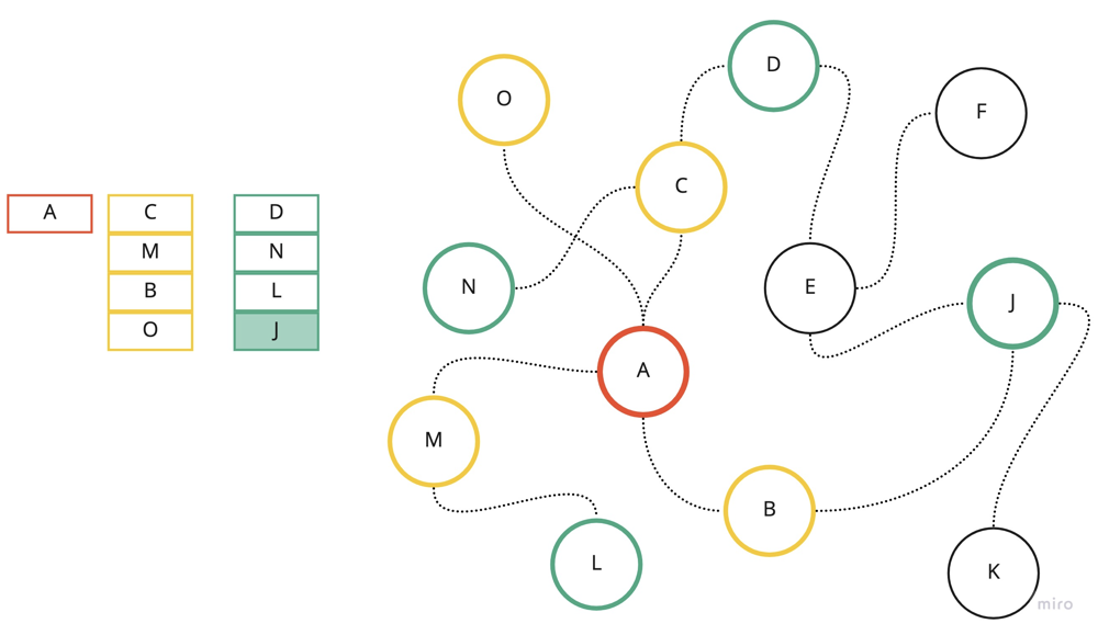
Visualization of BFS with first 3 layers. A - root node/first lavel, C/M/B/O - second layer, D/N/L/J - third layer.
- Algorithm uses queue for implementation.
- It checks whether a vertex has been explored before enqueueing the vertex.
- We can track if the node was already explored by modifying the original matrix.
- BFS algorithm can be instructed with additional array dist which can help to
track the parent node of the next node. This will help to reconstruct the path
by looping backward from end node.
DFS:
Is an algorithm for traversing or searching tree or graph data structures. The algorithm starts at the root node (selecting some arbitrary node as the root node in the case of a graph) and explores as far as possible along each branch before backtracking.
As BFS traverse wide, DFS goes deep. It starts from first node, and goes deep in a path till it traverse the leaf node/the last node before start traversing its next path.
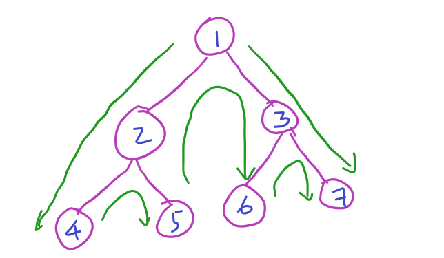
In the above tree, it first starts from root node 1, does deep to 2 and more deeper to 4. Node 4 has no children, so it is done with that path visits 5 and traverse back to 1 and starts visiting deep 3,6 and 7.
Further we can traverse in three different ways,
- Pre-Order: Visiting root first, left node next and finally right node.
- Inorder: Visiting left first, root node next and finally right node.
- Post-Order: Visiting left first, right node next and finally root node.
So the traversal of above tree is going to be,
Pre-Order: 1245367
Inorder: 4251637
Post-Order: 4526731
DFS of graph is also goes deep till it traverse all the nodes in the graph.
Implementation:
DFS: LIFO (Last In First Out)
We are going to get the help of stack, in order to traverse the tree/graph DFS way.
- Add the visited Node to stack.
- Pop the Node from stack, explore its children and add them to stack.
- Explore all the nodes till stack becomes empty.
Here we are going to see pre-order traversal of the below tree using stack. Same technique can be used to perform both inorder and post-order traversals just by changing the order of visiting nodes.
Question: Keys and Rooms
Description
There are n rooms labeled from 0 to n - 1 and all the rooms are locked except for room 0. Your goal is to visit all the rooms. However, you cannot enter a locked room without having its key.
When you visit a room, you may find a set of distinct keys in it. Each key has a number on it, denoting which room it unlocks, and you can take all of them with you to unlock the other rooms.
Given an array rooms where rooms[i] is the set of keys that you can obtain if you visited room i, return true if you can visit all the rooms, or false otherwise.
Example 1:
Input: rooms = [[1,3],[3,0,1],[2],[0]]
Output: false
Explanation: We can not enter room number 2 since the only key that unlocks it is in that room.
Example 2:
Input: rooms = [[1,3],[3,0,1],[0],[2]]
Output: true
Explanation: We visit room 0 and pick up key 1. We then visit room 1 and pick up key 3. We then visit room 3 and pick up key 2. We then visit room 3 and pick up key 0. Since we were able to visit every room, we return true.
Constraints:
n == rooms.length2 <= n <= 10000 <= rooms[i].length <= 10001 <= sum(rooms[i].length) <= 30000 <= rooms[i][j] < n- All the values of
rooms[i]are unique.
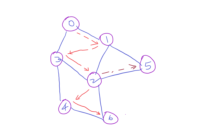
In above example,
- First we are visiting Node 1, add them to stack, explore its children and add its right child 3 first and then left child 2.
- Now the stack has nodes 2 and 3. Explore 2’s children and add its right child 5 and then its left child 4 to stack. And pop 2.
- Further pop nodes from stack and add its children until stack becomes empty.
Solution - The basic idea of the code is to keep a record of all the keys you have already obtained. - You can obtain all the keys in the rooms that you can go to - And if the count of all the keys you can obtain is equal to the number of rooms, your answer is True.
Code
from collections import deque
class Solution:
    def canVisitAllRooms(self, rooms):
        visited=[False]*len(rooms) #The visited array for the DFS to make sure we don't explore visited nodes again
        stack=deque() #The stack for carrying the BFS
        stack.append(0) #We know the root node is 0 since it is marked in the question, so we add it

        while(len(stack)>0): #DFS till stack is empty
            key=stack.pop()
            visited[key]=True #Marking node as visited, it can be done while adding into stack as well, like in the last question
            for j in rooms[key]: #Exploring all options, the keys found in the new room
                if(visited[j]==False):
                    stack.append(j)


        for i in visited:#If all rooms are visited the result is True, else False
            if(i==False):
                return False
        return True


Soln = Solution()
print(Soln.canVisitAllRooms([[1],[2],[3],[]]))
- Algorithm usually uses recursion implementation.
- We mark the node as visited and will keep exploring its neighbors if there are not yet explored.
- DFS can be useful to find connected components. We can iterate through the nodes and call dfs() to find all nodes which belongs to component.
- We can use unordered_map
Minimum Spanning Tree (Prim's Algorithm):
Minimum Spanning Tree (MST) is a spanning tree with least possible edge weight. What that means is that it is an undirected graph, where all the vertices are connected, with least possible edge weight, and no cycles. A weighted, undirected, and connected graph can have many spanning trees but only one MST.
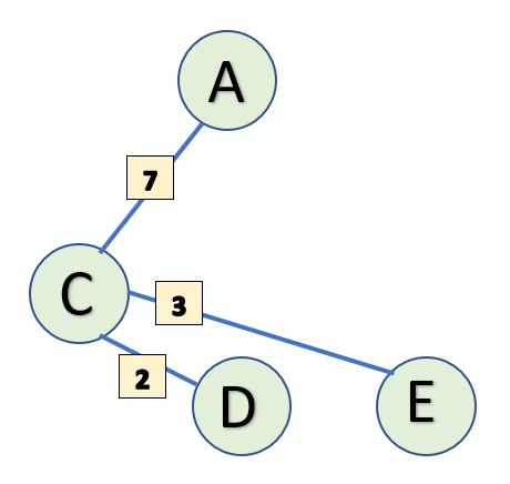
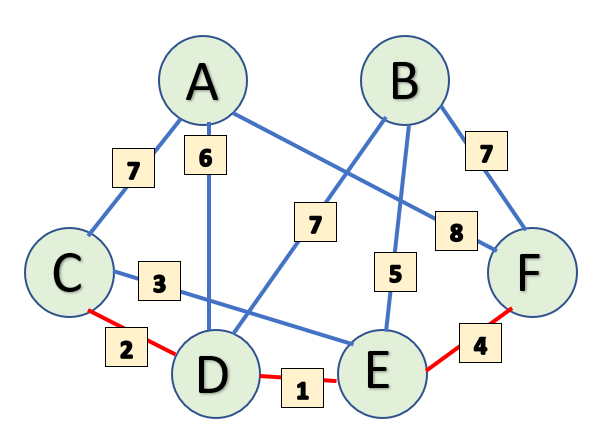
Here is an image of a weighted, undirected, and connected graph. Blue edges are all the spanning trees of this graph and red edges are the minimum spanning tree (We will only use MST for all the future explanations in this guide.)
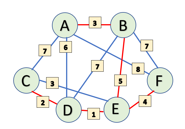
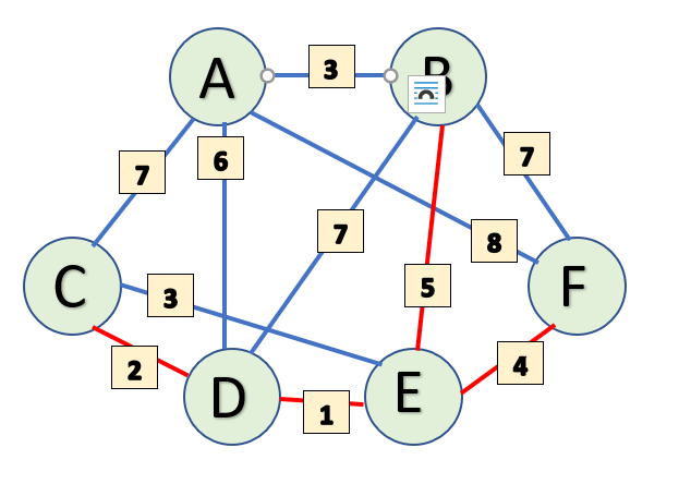
The total number of vertices, V in this Graph are 6. The total number of edges, E in an MST is (V-1) i.e. 6-1=5 edges. This is what the MST looks like for the above graph-
Alright, now that we have a basic understanding of how MST is supposed to be, let’s try and understand how to find a minimum spanning tree when given a graph!
Prim's Algorithm
Prim’s algorithm is a greedy algorithm. To find the MST using Prim’s, we pick an initial starting vertex and add it to a set. Then we grow the MST from that initial vertex by adding adjacent vertices one by one based on least value of edge weight.
Let’s create 2 disjoint (no common value) subsets of vertices, one is called StartSet and the other is called MstSet. StartSet is a key value pair with vertices and their distances from the adjacent vertix that has been added to the MstSet.
In the beginning, StartSet has all the vertices and MstSet has nothing.
StartSet: {(A, INF), (B, INF), (C, INF), (D, INF), (E, INF), (F, INF)}
MstSet: {}
Let’s pick a starting point. It doesn’t matter which one because MST is unique and no matter where you start, you are going to end up with the same tree.
I will begin at vertex C. From vertex C, we have the following paths-
Since we picked our starting point, let's add vertex C to MstSet and update it's value to 0 in StartSet (as it is our initial vertex and distant from a node to itself is 0.
Also update the values of vertices adjacent to C with their distances from C. Since A, D and E are adjacent to C, their values in StartSet are updated. Our subsets look as follows-
StartSet: {(A, 7), (B, INF), (C, 0), (D, 2), (E, 3), (F, INF)}
MstSet: {C}
From C, we can either pick A, D, or E as our next vertex.
Since the Prim's algorithm is Greedy, it will choose the path of least value i.e. the edge between C and D and will add vertex D to MstSet.
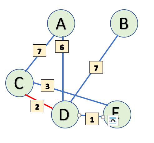
Next, the same process repeats with D. Update the value of vertices adjacent to D in StartSet. One thing to note here is that the distance of A from D is 6 which is less than distance of A from C. Therefore, in our subset StartSet, the value of A will update to 6 from 7. Same goes for E whose value will be updated from 3 to 1.
Let's look at the values in our subsets-
StartSet: {(A, 6), (B, 7), (C, 0), (D, 2), (E, 1), (F, INF)}
MstSet: {C, D}
So far we have C and D in our MST. Let's grow our MST some more by picking the next vertex.
Now our edge values are 6, 7 and 1. Since 1 is smallest, the next vertex to be added to the MstSet will be E. You can also look at our subsets and see that out of all the vertices that are currently not in MstSet, E has the least value.
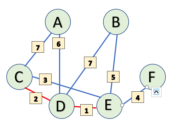
Continuing our tradition of updating adjacent vertices in StartSet, B is updated to 5 and F is updated to 4.
Our subsets currently look like this-
StartSet: {(A, 6), (B, 5), (C, 0), (D, 2), (E, 1), (F, 4)}
MstSet: {C, D, E}
Now we may have a problem! The values of edges coming from E are 3, 4 and 5. Since 3 is smaller than the 2, ideally we should pick that. However, we can't do that because C is already in MstSet. So we will go a step further and pick the edge with value 4 i.e. the E-F edge.
Once again, add F to MstSet and update the adjacent vertices' values.
There is no change of values for vertices adjacent to F.
Let's take a quick look at our subsets after adding F.
StartSet: {(A, 6), (B, 5), (C, 0), (D, 2), (E, 1), (F, 4)}
MstSet: {C, D, E, F}
Now the only vertices that are not in MstSet are A and B. As you can see from the subset, between A and B, B has the smaller value (5). Also in the graph, the least value of edge weight to reach B is 5 (E-B edge) as compared to A which is 7 (F-A edge).
Therefore, we will go ahead and add B to our MstSet and update the values of it's adjacent vertices.
Value of A is updated to 3.
Our subsets look like this-
StartSet: {(A, 3), (B, 5), (C, 0), (D, 2), (E, 1), (F, 4)}
MstSet: {C, D, E, F, B}
Now, only A needs to be added. As we can see from both the graph and the subset, the least cost way to reach A is through A-B edge.
So, we will add A to our MstSet.
Let's look at the final values of our subsets-
StartSet: {(A, 3), (B, 5), (C, 0), (D, 2), (E, 1), (F, 4)}
MstSet: {C, D, E, F, B, A}
All the vertices have been added to the MstSet!
And finally, we have our Minimum Spanning Tree.

Question: Optimized water distribution in a village
Description
There are n houses in a village. We want to supply water for all the houses by building wells and laying pipes.
For each house i, we can either build a well inside it directly with cost wells[i], or pipe in water from another well to it. The costs to lay pipes between houses are given by the array pipes, where each pipes[i] = [house1, house2, cost] represents the cost to connect house1 and house2 together using a pipe. Connections are bidirectional.
Find the minimum total cost to supply water to all houses.
Example 1:
Input: n = 3, wells = [1,2,2], pipes = [[1,2,1],[2,3,1]]
Output: 3
Explanation: The image shows the costs of connecting houses using pipes. The best strategy is to build a well in the first house with cost 1 and connect the other houses to it with cost 2 so the total cost is 3.
Constraints:
- 1 <= n <= 10000
- wells.length == n
- 0 <= wells[i] <= 10^5
- 1 <= pipes.length <= 10000
- 1 <= pipes[i][0], pipes[i][1] <= n
- 0 <= pipes[i][2] <= 10^5
- pipes[i][0] != pipes[i][1]
example 1 pic:
Code
from collections import deque
import collections
import heapq
class Solution:
    def minCostToSupplyWater(self, n, wells, pipes):
        c = collections.defaultdict(list) #First step is creating the adjacency list to represent the graph

        #The question as of now is not in MST since nodes value cost as well, this can be converted to MST by adding a base node
        #This base node will have edge with every node with a weight equivalent to the cost of that node, and will also serve as the root node
        for i, cost in enumerate(wells, 1): #Adding all the edges to the base node, cost equal to cost of well
            c[0].append((cost, i))
            c[i].append((cost, 0))
        for i, j, cost in pipes: #Adding all other edges as adjacency list, cost first so it can be used in a heap
            c[i].append((cost, j))
            c[j].append((cost, i))

        ans, visited, heap = 0, [0] * (n+1), c[0] #Answer is the final minimum cost, visited is the visited array, heap is to carry the Prim's
        visited[0] = 1 #Starting with the root, our case the node we added, node 0
        heapq.heapify(heap)
        while heap:
            d, j = heapq.heappop(heap)
            if not visited[j]: #Only visiting unvisited nodes
                visited[j], cnt, ans = 1, cnt+1, ans+d #For adding to our heap, each edge adds to the cost of the spanning tree
                for record in c[j]: heapq.heappush(heap, record) #Adding the new node to our heap
        return ans


Soln = Solution()
print(Soln.minCostToSupplyWater(3, [1,2,2], [[1,2,1],[2,3,1]]))
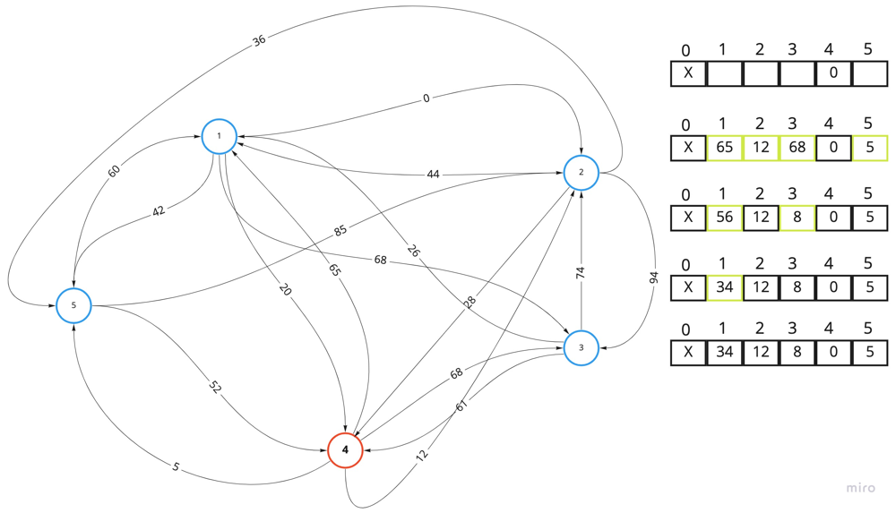
Dijkstra's algorithm:
Is an algorithm for finding the shortest paths between nodes in a graph, which may represent, for example, road networks.
Dijkstra's algorithm is a Single-Source-Shortest-Path algorithm, which means that it calculates shortest distance from one vertex to all the other vertices.
The node from where we want to find the shortest distance is known as the source node. For the rest of the tutorial, I'll always label the source node as S. And the distance to source node is naturally going to be zero.
So, if we had an array of distances called dist[] and source node is 2 then dist[] would be
[INF, INF, 0, INF, INF]
  0    1   2   3    4
// Consider INF as infinity since we don't know what the actual distance is. But we are very much sure that the distance to the source node is 0.
Let's start.
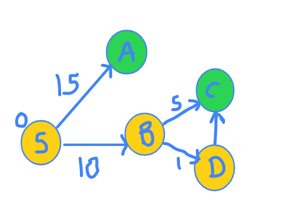
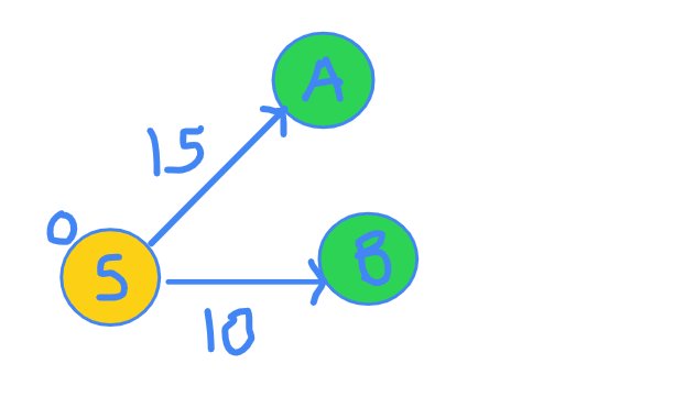
Have a look at the image below. We shall work with it in this tutorial.
Remember what I said about the source node? I said that we were SURE that the shortest distance to source node is going to be zero. Do you agree with me on that point? Of course, yes, because there was no path to travel.
What does the distance array for our graph look like?
Node     |  S   A   B   C   D
Distance |  0  INF INF INF INF
Let's break the problem. Let's rip apart this graph.
We are at S currently. Let's see where we can go from S.

You are at node S. There are 2 edges that come out of S. One edge goes to A and other goes to B. Edge SA distance is 15 and edge SB distance if 10. You can clearly verify this in the figure.
I now claim that I am SURE that the shortest distance to B is 10. Why though? How many other ways are possible, through which you can reach to node B? Maybe there will be some edge from A to B. But since distance to A is already 15, any edge from A to B will only increase that distance and will never be able to become less than 10. This is the most important step. Read it again if you did not get it.
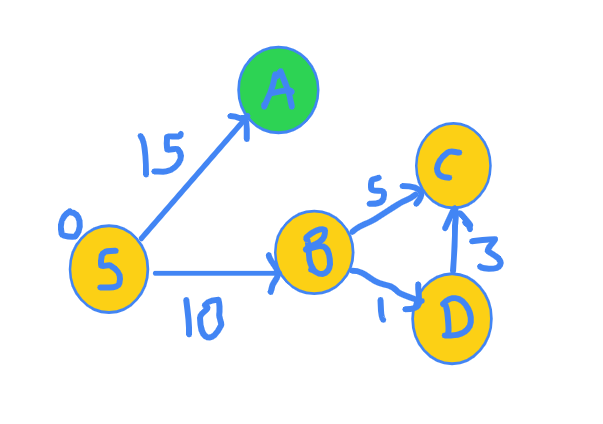
Now, that I am SURE of the shortest distance to reach B, I discover more vertices from B.
Now, our exploration graph looks something like this.
and the distance array has been updated.
Node     |  S   A   B   C   D
Distance |  0  INF  10 INF INF
Let's see what the current scenario looks like.
Nodes for which we know the shortest distance: S and B.
What are we looking at now?
At all the nodes we can reach from the S and B.
Again, the same question. Which node's shortest distance can we be SURE of ?
I claim it's node D.
Look at the figure again.

The distance to D is 10 + 1 = 11, and no other path can have length smaller than this since their own distances are greater than 11.
Hence, we now include D in our set of vertices for which shortest distances is known. Also, we explore more edges going from node D.
Note that we are always picking the green vertex with the minimum distance.
So, now our exploration graph looks something like this.
Distance has been updated.
Node     |  S   A   B   C   D
Distance |  0  INF  10 INF  11
Now, same question. Which node's shortest distance can we be SURE of? More specifically. Which green node's shortest distance can we be SURE of? Yes, right. It is C because the path S-B-D-C gives distance of 10 + 1 + 3 = 14 which is the lowest.
Hence, we include C into the set of nodes for which final distance have been finalized and we also explore it's neighbours.
The exploration graph now looks like this.
Distance has been updated again.
Node     |  S   A   B   C   D
Distance |  0  INF  10  14  11
Again, for which node are we SURE of? There is just one node remaining and so it is the shortest. So, we include it in the set of nodes whose final distances are known and explore it's neighbours.
Now, the exploration graph is as follows:
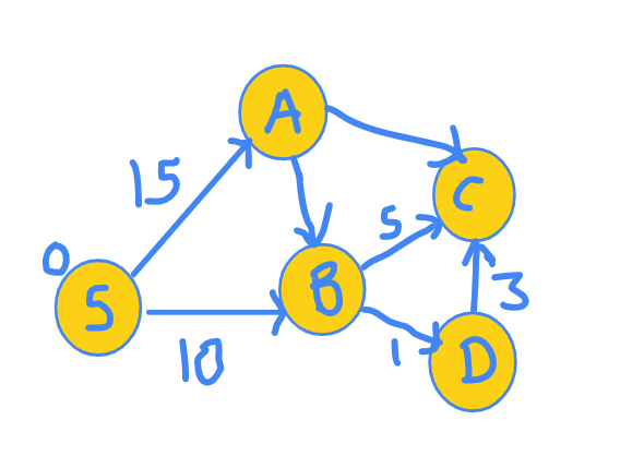
Final distance array now looks like this:
Node     |  S   A   B   C   D
Distance |  0  15  10  14  11
But now, since we have no green nodes, we stop. We have visited all the nodes.
Couple of key points here. How were we SURE of the shortest distance of a green node? That node had the shortest distance among all the other green nodes.
Now, summarizing Djikstra's algorithm:
- We keep a set of vertices for which final shortest distance is already known to us. Initially only the source vertex S belongs to this set.
- We do several iterations, during which we pick the green node with the minimum distance and add it to the set of vertices whose distances are finalized and also all nodes reaching from this node and not VISITED (i.e. NOT MARKED YELLOW), are made green.
And that's it. That's the working of Djikstra's algorithm.
Regarding the implementation, since we need the node with minimum distance, a min-heap is prefered. Implementations with sets( the ones based on BSTs) are also popular. You can find the implementations online with both the data structures.
Now, for a moment, let's go back to where we started.
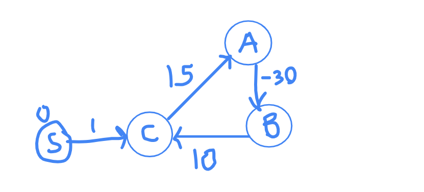
At this point, we chose B. So, what we have done is finalized the distance to B and it can never be changed in coming iterations. Now, let's say that there was an edge from A to B with cost as -10 (Negative ten). The distance then is 15 + (-10) = 5, which is lower than 10.
But, we had said that it can never be less than 10. Then, how come this?
Here is the truth. Djikstra's algorithm doesn't work for negative edge weights.
Let's think about the graphs involving negative weights cycles. If there is a negative weight cycle like the C-A-B-C below, we can keep moving in cycles and each iteration of the cycle will decrease the distance, so negative weight cycle is a big NO for Djikstra.
It's intuitive to understand that Djikstra doesn't work for negative cycles but not very intuitive to understand why it doesn't work for negative edges with no negative cycles.
Question : Network Delay Time
You are given a network of n nodes, labeled from 1 to n. You are also given times, a list of travel times as directed edges times[i] = (ui, vi, wi), where ui is the source node, vi is the target node, and wi is the time it takes for a signal to travel from source to target.
We will send a signal from a given node k. Return the minimum time it takes for all the n nodes to receive the signal. If it is impossible for all the n nodes to receive the signal, return -1.
Example 1:

Input: times = [[2,1,1],[2,3,1],[3,4,1]], n = 4, k = 2
Output: 2
Example 2:
Input: times = [[1,2,1]], n = 2, k = 1
Output: 1
Example 3:
Input: times = [[1,2,1]], n = 2, k = 2
Output: -1
Constraints:
1 <= k <= n <= 1001 <= times.length <= 6000times[i].length == 31 <= ui, vi <= nui != vi0 <= wi <= 100- All the pairs
(ui, vi)are unique. (i.e., no multiple edges.)
Solution:
import heapq
class Solution:
    def networkDelayTime(self, times, n, k):
        #create adjacency list
        adjList = {i:[] for i in range(1, n+1)} #Format of the adjacency list node: [neighbour, weight]
        for src, dest, weight in times:
            adjList[src].append([dest, weight])
        #create minHeap
        minHeap = []
        minHeap.append([0, k]) #Minheap is of the structure distance, node; Initial is 0,k since k is starting node as written in question and its at 0 distance from itself
        heapq.heapify(minHeap)
        #dikjstra
        dist = [float("inf")] * (n+1) #Initial distance to all nodes is infinite
        dist[k] = 0 #Distance to the starting node set to zero since it is the starting node itself
        while minHeap: #Minheap to implement the jijkstras
            dis, node = heapq.heappop(minHeap)
            for it in adjList[node]:
                edgeWeight = it[1]
                edgeNode = it[0]
                if (dis+edgeWeight) < dist[edgeNode]: #Applying the formula to update the distance array
                    dist[edgeNode] = dis+edgeWeight
                    heapq.heappush(minHeap, [dist[edgeNode], edgeNode]) #Since the node is visited now, we add it to our heap
        #result
        return max(dist[1:]) if max(dist[1:]) != float("inf") else -1 #Max of all the latency, else -1 if not possible

Soln = Solution()
print(Soln.networkDelayTime([[2,1,1],[2,3,1],[3,4,1]], 4, 2))
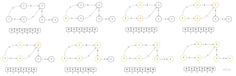
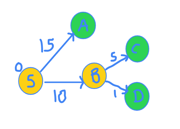
Visualization of traversing graph using Dijkstra algorithm and distance array. The priority queue itself is not shown there, as well as redundant nodes that we might have in priority queue. Green node - explored/current node, Yellow - node in the priority queue.
Notes:
- We will have a set to track visited nodes.
- We will create a distance array to track the distance to each node. Initial node will have 0, others maximum. There is a room for optimization: if the node we got from the pq has larger cost than in our dist[] array, we should not explore it as we already got a better option.
- We will use min priority_queue to get the node with the minimum distance from the current node.
- If we are only interested in shortes distance till some END node, we can terminate the search earlier: if (node == dst) return cost;
- If we already find a better path we shouldn't explore it further: if (dist[node] < stops) continue;
Extra Graph Algorithms:
Union-Find:
Union–find data structure or disjoint-set data structure or merge–find set, is a data structure that stores a collection of disjoint (non-overlapping) sets. Equivalently, it stores a partition of a set into disjoint subsets. It provides operations for adding new sets, merging sets (replacing them by their union), and finding a representative member of a set. Helps to find the number of connected components, and can help to find MST.
class UnionFind {
    public:
    UnionFind(int n) : parent(n) {
        iota(parent.begin(), parent.end(), 0);
    }

    int Find(int x) {
        int temp = x;
        while (temp != parent[temp]) {
            temp = parent[temp];
        }
        // Path compression below
        while (x != temp) {
            int next = parent[x];
            parent[x] = temp;
            x = next;
        }
        return x;
    }

    void Union(int x, int y) {
        int xx = Find(x);
        int yy = Find(y);
        if (xx != yy) {
            parent[xx] = yy;
        }
    }

    private:
           vector<int> parent;
};
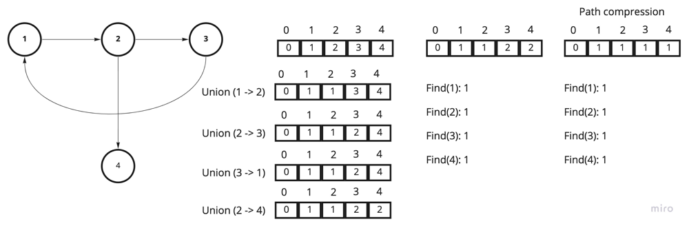
The above picture demonstrates the state of the parent array after multiple Union() calls, follows multiple Find() calls.
Notes:
1. We can use vector to hold the set of nodes or unordered_map
2. If the parent[id] == id, we know that id is the root node.
3. The data structure using two methods Union() - union to nodes/components, and Find() - find the root node.
4. We can do path compression, so after some number of Find() calls it will be O(1) to call Find() again.
Minimum Spanning Tree (Union Find):
A minimum spanning tree (MST) is a subset of the edges of a connected, edge-weighted undirected graph that connects all the vertices together, without any cycles and with the minimum possible total edge weight.
Solution for Connecting Cities With Minimum Cost: https://leetcode.com/problems/connecting-cities-with-minimum-cost/.
class UnionFind {
public:
    UnionFind(int n) : parent(n) {
          iota(parent.begin(), parent.end(), 0);
    }
    int Find(int x) {
        int temp = x;
        while (temp != parent[temp]) {
            temp = parent[temp];
        }
        while (x != temp) {
            int next = parent[x];
            parent[x] = temp;
            x = next;
        }
        return temp;
    }
    bool Union(int x, int y) {
        int xx = Find(x);
        int yy = Find(y);
        if (xx == yy) return false;
        parent[xx] = yy;
        return true;
    }

private:
    vector<int> parent;
};
int minimumCost(int n, vector<vector<int>>& connections) {
    sort(connections.begin(), connections.end(), [](const auto& lhs, const auto& rhs){
        return lhs[2] < rhs[2];
    });
    UnionFind uf(n + 1);
    int sum = 0, count = 0;
    for (auto& c : connections) {
        if (uf.Union(c[0], c[1])) {
            count++;
            sum += c[2];
        }
        if (count == n - 1) return sum; // Return earlier once graph is connected.
    }
    return -1;
}
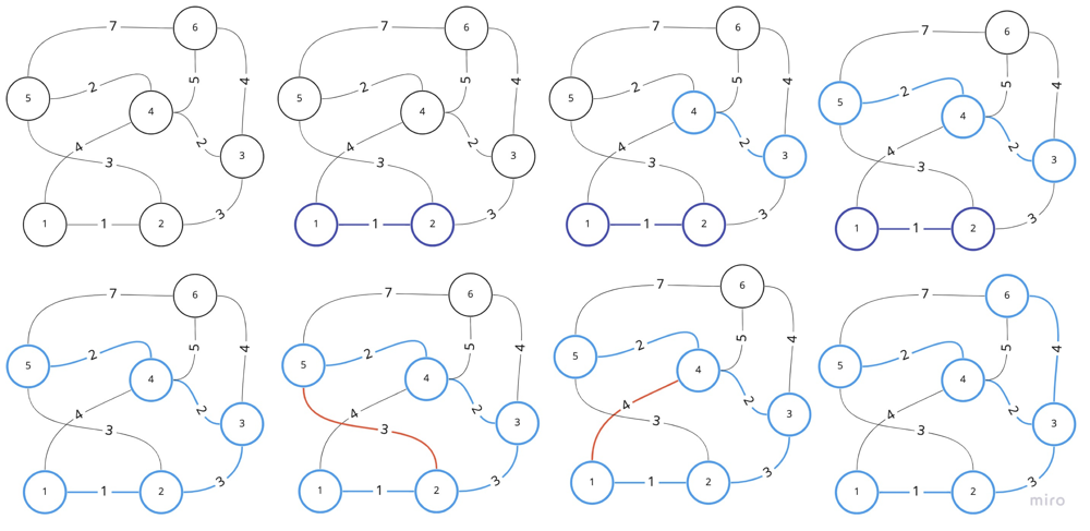
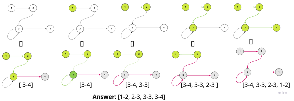
Visualization of Kruskal's algorithm: we will try to union nodes if they are not connected.
Notes:
1. One of the implementation of MST algorithm use Union Find algorithm (Kruskal's Algorithm).
2. We need to sort elements by the weight before appying the algorithm, or we can use min priority_queue.
Topological sort:
Is a linear ordering of its vertices such that for every directed edge uv from vertex u to vertex v, u comes before v in the ordering.
    // Kahn's Algorithm
    vector<vector<int>> adj(numCourses);
    vector<int> indegree(numCourses, 0);
    for (auto& p : prerequisites) {
        indegree[p[1]]++;
        adj[p[0]].push_back(p[1]);
    }
    queue<int> q;
    for (int i = 0; i < numCourses; i++) {
        if (indegree[i] == 0) q.push(i);
    }
    int prereq = 0;
    while (!q.empty()) {
        int el = q.front();
        q.pop();
        prereq++;
        for (auto& next : adj[el]) {
            if (--indegree[next] == 0) {
                q.push(next);
            }
        }
    }
    return prereq == numCourses;
The above picture demonstrates linear order of the given graph. The vertices can be tasks, and edges can represent some contraints, such as U should be finished before V in (U -> V).
Notes:
1. We will have the indegree array to count, which nods should be visited first.
2. We will have a queue to push the nodes that don't have any dependencies.
Bellman Ford:
Is an algorithm that computes shortest paths from a single source vertex to all of the other vertices in a weighted digraph.
class Solution {
public:
    int networkDelayTime(vector<vector<int>>& times, int n, int k) {
        vector<int> dist(n + 1, INT_MAX);
        dist[k] = 0;
        for (int i = 1; i <= n; i++) {
            for (auto& t : times) {
                if (dist[t[0]] != INT_MAX && dist[t[1]] > dist[t[0]] + t[2]) {
                    dist[t[1]] = dist[t[0]] + t[2];
                }
            }
        }
        int res = 0;
        for (int i = 1; i <= n; i++) {
            res = max(res, dist[i]);
        }
        return res == INT_MAX ? -1 : res;
    }
};
The above picture demonstrates how the dist array incrementally updated with better values. If not a single value is updated during iteration - we can stop earlier.
Notes:
1. We will use the array to hold the distance between particular start node and all others.
2. We will try to improve distance n times between all nodes in the graph.
Floyd Warshall:
Is an algorithm for finding shortest paths in a directed weighted graph with positive or negative edge weights.
class Solution {
public:
    int networkDelayTime(vector<vector<int>>& times, int n, int k) {
        vector<vector<long>> dist(n, vector<long>(n, INT_MAX));
        for (auto& t : times)
            dist[t[0] - 1][t[1] - 1] = t[2];
        for (int i = 0; i < n; i++)
            dist[i][i] = 0;
        for (int k = 0; k < n; k++) {
            for (int i = 0; i < n; i++) {
                for (int j = 0; j < n; j++) {
                    dist[i][j] = min(dist[i][j], dist[i][k] + dist[k][j]);
                }
            }
        }
        long res = INT_MIN;
        for (int i = 0; i < n; i++) {
            if (dist[k - 1][i] == INT_MAX) return -1;
            res = max(res, dist[k - 1][i]);
        }
        return (int)res;
    }
};
Vizualization for Floyd Warshall is slightly different from Bellman Ford, but the idea stays the same.
Notes:
1. We will use vector
2. We will have a 3 loops, checks if we can improve the distance between i and j by using k node.
Eulearian Path:
Is an algorithm that finds a path that uses every edge in a graph only once.
The algorithm below is a solution for the "Reconstruct Itinerary": https://leetcode.com/problems/reconstruct-itinerary/
class Solution {
public:
    void dfs(unordered_map<string, multiset<string>>& graph,
             vector<string>& res, string start) {
        while (graph[start].size() > 0) {
            auto next = *graph[start].begin();
            graph[start].erase(graph[start].begin());
            dfs(graph, res, next);
        }
        res.push_back(start);
    }
    vector<string> findItinerary(vector<vector<string>>& tickets) {
        unordered_map<string, multiset<string>> graph;
        for (const auto& t : tickets) graph[t[0]].insert(t[1]);
        vector<string> res;
        dfs(graph, res, "JFK");
        reverse(res.begin(), res.end());
        return res;
    }
};
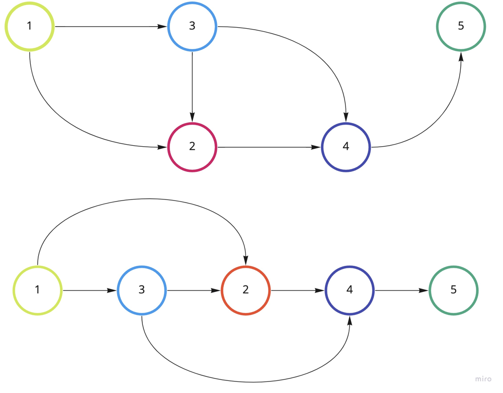
The above picture is the visualization of eulerian path algorithm. You can observe how the result is constructed on the backtracking.
Notes:
1. The algorithm almost identical to the dfs traversal with one main instrumentation: we are building the path on the backtrack of the dfs algorithm: res.push_back(start);
2. That is why we should reverse the list at the end of the traversal: reverse(res.begin(), res.end());
3. In the above implementation we are using multiset (because of the problem), but the general implementation may use vector<> and additional vector<> to track the outgoing degrees, and use it for two main purposes: as index in the adj list, and to track how many node we not visited yet.